Example 12-5: Poverty and Teen Birth Rate Data Section
(Data source: The U.S. Census Bureau and Mind On Statistics, (3rd edition), Utts and Heckard). In this example, the observations are the 50 states of the United States (Poverty data - Note: remove data from the District of Columbia). The variables are y = percentage of each state’s population living in households with income below the federally defined poverty level in the year 2002, \(x_{1}\) = birth rate for females 15 to 17 years old in 2002, calculated as births per 1000 persons in the age group, and \(x_{2}\) = birth rate for females 18 to 19 years old in 2002, calculated as births per 1000 persons in the age group.
The two x-variables are correlated (so we have multicollinearity). The correlation is about 0.95. A plot of the two x-variables is given below.
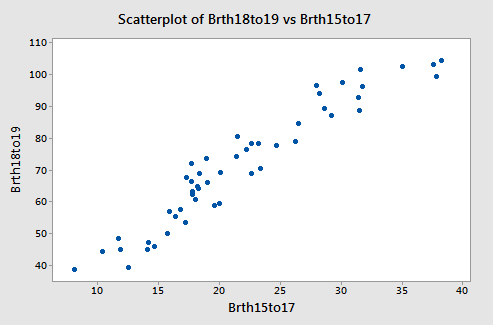
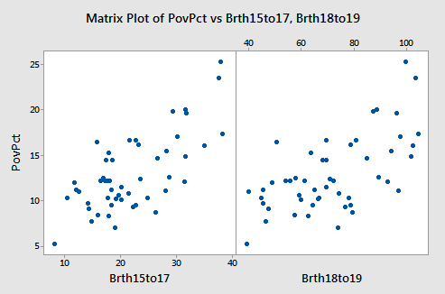
The figure below shows plots of y = poverty percentage versus each x-variable separately. Both x-variables are linear predictors of the poverty percentage.
Minitab results for the two possible simple regressions and the multiple regression are given below.
Regression Analysis: PovPct versus Brth15to17
Regression Equation
\(\widehat{PovPct} = 4.49 + 0.387 Brth15to17\)
| Predictor | Coef | SE Coef | T | P |
|---|---|---|---|---|
| Constant | 4.487 | 1.318 | 3.40 | 0.001 |
| Brth15to17 | 0.38718 | 0.05720 | 6.77 | 0.000 |
S = 2.98209 R-Sq = 48.8% R-Sq(adj) = 47.8%
Regression Analysis: PovPct versus Brth18to19
Regression Equation
\(\widehat{PovPct} = 3.05 + 0.138 Brth18to19\)
| Predictor | Coef | SE Coef | T | P |
|---|---|---|---|---|
| Constant | 3.053 | 1.832 | 1.67 | 0.102 |
| Brth18to19 | 0.13842 | 0.02482 | 5.58 | 0.000 |
S = 3.24777 R-Sq = 39.3% R-Sq(adj) = 38.0%
Regression Analysis: PovPct versus Brth15to17, Brth18to19
Regression Equation
\(\widehat{PovPct} = 6.44 + 0.632 Brth15to17 - 0.102 Brth18to19\)
| Predictor | Coef | SE Coef | T | P |
|---|---|---|---|---|
| Constant | 6.440 | 1.959 | 3.29 | 0.002 |
| Brth15to17 | 0.6323 | 0.1918 | 3.30 | 0.002 |
| Brth18to19 | -0.10227 | 0.07642 | -1.34 | 0.187 |
s = 2.95782 R-Sq = 50.7% R-Sq(adj) = 48.6%
We note the following:
- The value of the sample coefficient that multiplies a particular x-variable is not the same in the multiple regression as it is in the relevant simple regression.
- The \(R^{2}\) for the multiple regression is not the sum of the \(R^{2}\) values for the simple regressions. An x-variable (either one) is not making an independent “add-on” in the multiple regression.
- The 18 to 19-year-old birth rate variable is significant in the simple regression but is not in the multiple regression. This discrepancy is caused by the correlation between the two x-variables. The 15 to 17-year-old birth rate is the stronger of the two x-variables and given its presence in the equation, the 18 to 19-year-old rate does not improve \(R^{2}\) enough to be significant. More specifically, the correlation between the two x-variables has increased the standard errors of the coefficients, so we have less precise estimates of the individual slopes.