Example 6-1: Heart attacks in Rabbits Section
Let's investigate an example that highlights the differences between the three hypotheses that we will learn how to test in this lesson.
When the heart muscle is deprived of oxygen, the tissue dies and leads to a heart attack ("myocardial infarction"). Apparently, cooling the heart reduces the size of the heart attack. It is not known, however, whether cooling is only effective if it takes place before the blood flow to the heart becomes restricted. Some researchers (Hale, et al, 1997) hypothesized that cooling the heart would be effective in reducing the size of the heart attack even if it takes place after the blood flow becomes restricted.
To investigate their hypothesis, the researchers conducted an experiment on 32 anesthetized rabbits that were subjected to a heart attack. The researchers established three experimental groups:
- Rabbits whose hearts were cooled to 6º C within 5 minutes of the blocked artery ("early cooling")
- Rabbits whose hearts were cooled to 6º C within 25 minutes of the blocked artery ("late cooling")
- Rabbits whose hearts were not cooled at all ("no cooling")
At the end of the experiment, the researchers measured the size of the infarcted (i.e., damaged) area (in grams) in each of the 32 rabbits. But, as you can imagine, there is great variability in the size of hearts. The size of a rabbit's infarcted area may be large only because it has a larger heart. Therefore, in order to adjust for differences in heart sizes, the researchers also measured the size of the region at risk for infarction (in grams) in each of the 32 rabbits.
With their measurements in hand (Cool Hearts data), the researchers' primary research question was:
Does the mean size of the infarcted area differ among the three treatment groups — no cooling, early cooling, and late cooling — when controlling for the size of the region at risk for infarction?
A regression model that the researchers might use in answering their research question is:
\(y_i=(\beta_0+\beta_1x_{i1}+\beta_2x_{i2}+\beta_3x_{i3})+\epsilon_i\)
where:
- \(y_{i}\) is the size of the infarcted area (in grams) of rabbit i
- \(x_{i1}\) is the size of the region at risk (in grams) of rabbit i
- \(x_{i2}\) = 1 if early cooling of rabbit i, 0 if not
- \(x_{i3}\) = 1 if late cooling of rabbit i, 0 if not
and the independent error terms \(\epsilon_{i}\) follow a normal distribution with mean 0 and equal variance \(σ^{2}\).
The predictors \(x_{2}\) and \(x_{3}\) are "indicator variables" that translate the categorical information on the experimental group to which a rabbit belongs into a usable form. We'll learn more about such variables in Lesson 8, but for now observe that for "early cooling" rabbits \(x_{2}\) = 1 and \(x_{3}\) = 0, for "late cooling" rabbits \(x_{2}\) = 0 and \(x_{3}\) = 1, and for "no cooling" rabbits \(x_{2}\) = 0 and \(x_{3}\) = 0. The model can therefore be simplified for each of the three experimental groups:
| Early Cooling | \(y_i=(\beta_0+\beta_1x_{i1}+\beta_2)+\epsilon_i\) |
|---|---|
| Late Cooling | \(y_i=(\beta_0+\beta_1x_{i1}+\beta_3)+\epsilon_i\) |
| No Cooling | \(y_i=(\beta_0+\beta_1x_{i1})+\epsilon_i\) |
Thus, \(\beta_2\) represents the difference in the mean size of the infarcted area — controlling for the size of the region at risk —between "early cooling" and "no cooling" rabbits. Similarly, \(\beta_3\) represents the difference in the mean size of the infarcted area — controlling for the size of the region at risk —between "late cooling" and "no cooling" rabbits.
Fitting the above model to the researchers' data, Minitab reports:
Regression Equation
Inf = -0.135 + 0.613 Area - 0.2435 X2 - 0.0657 X3
A plot of the data adorned with the estimated regression equation looks like this:
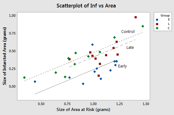
The plot suggests that, as we'd expect, as the size of the area at risk increases, the size of the infarcted area also tends to increase. The plot also suggests that for this sample of 32 rabbits with a given size of area at risk, 1.0 grams for example, the average size of the infarcted area differs for the three experimental groups. But, the researchers aren't just interested in this sample. They want to be able to answer their research question for the whole population of rabbits.
How could the researchers use the above regression model to answer their research question? Note that the estimated slope coefficients \(b_{2}\) and \(b_{3}\) are -0.2435 and -0.0657, respectively. If the estimated coefficients \(b_{2}\) and \(b_{3}\) were instead both 0, then the average size of the infarcted area would be the same for the three groups of rabbits in this sample. It can be shown that the mean size of the infarcted area would be the same for the whole population of rabbits — controlling for the size of the region at risk — if the two slopes \(\beta_{2}\) and \(\beta_{3}\) simultaneously equal 0. That is, the researchers's question reduces to testing the hypothesis \(H_{0}\colon \beta_{2} = \beta_{3} = 0\).
I'm hoping this example clearly illustrates the need for being able to "translate" a research question into a statistical procedure. Often, the procedure involves four steps, namely:
- formulating a multiple regression model
- determining how the model helps answer the research question
- checking the model
- and performing a hypothesis test (or calculating a confidence interval)
In this lesson, we learn how to perform three different hypothesis tests for slope parameters in order to answer various research questions. Let's take a look at the different research questions — and the hypotheses we need to test in order to answer the questions — for our heart attacks in rabbits example.
A research question Section
Consider the research question: "Is a regression model containing at least one predictor useful in predicting the size of the infarct?" Are you convinced that testing the following hypotheses helps answer the research question?
- \(H_{0}\colon \beta_{1} = \beta_{2} = \beta_{3} = 0\)
- \(H_{A}\colon\) At least one \(\beta_{i} \ne 0\) (for i = 1, 2, 3)
In this case, the researchers are interested in testing that all three slope parameters are zero. We'll soon see that the null hypothesis is tested using the analysis of variance F-test.
Another research question Section
Consider the research question: "Is the size of the infarct significantly (linearly) related to the area of the region at risk?" Are you convinced that testing the following hypotheses helps answer the research question?
- \(H_{0} \colon \beta_{1} = 0\)
- \(H_{A} \colon \beta_{1} ≠ 0\)
In this case, the researchers are interested in testing that just one of the three slope parameters is zero. You already know how to do this, don't you? Wouldn't this just involve performing a t-test for \(\beta_{1}\)? We'll soon learn how to think about the t-test for a single slope parameter in the multiple regression framework.
A final research question Section
Consider the researcher's primary research question: "Is the size of the infarct area significantly (linearly) related to the type of treatment after controlling for the size of the region at risk for infarction?" Are you convinced that testing the following hypotheses helps answer the research question?
- \(H_{0} \colon \beta_{2} = \beta_{3} = 0\)
- \(H_{A} \colon\) At least one \(\beta_{i} ≠ 0\) (for i = 2, 3)
In this case, the researchers are interested in testing whether a subset (more than one, but not all) of the slope parameters are simultaneously zero. We will learn a general linear F-test for testing such a hypothesis.
Unfortunately, we can't just jump right into the hypothesis tests. We first have to take two side trips — the first one to learn what is called "the general linear F-test."