The method of ordinary least squares assumes that there is constant variance in the errors (which is called homoscedasticity). The method of weighted least squares can be used when the ordinary least squares assumption of constant variance in the errors is violated (which is called heteroscedasticity). The model under consideration is
\(\begin{equation*} \textbf{Y}=\textbf{X}\beta+\epsilon^{*}, \end{equation*}\)
where \(\epsilon^{*}\) is assumed to be (multivariate) normally distributed with mean vector 0 and nonconstant variance-covariance matrix
\(\begin{equation*} \left(\begin{array}{cccc} \sigma^{2}_{1} & 0 & \ldots & 0 \\ 0 & \sigma^{2}_{2} & \ldots & 0 \\ \vdots & \vdots & \ddots & \vdots \\ 0 & 0 & \ldots & \sigma^{2}_{n} \\ \end{array} \right) \end{equation*}\)
If we define the reciprocal of each variance, \(\sigma^{2}_{i}\), as the weight, \(w_i = 1/\sigma^{2}_{i}\), then let matrix W be a diagonal matrix containing these weights:
\(\begin{equation*}\textbf{W}=\left( \begin{array}{cccc} w_{1} & 0 & \ldots & 0 \\ 0& w_{2} & \ldots & 0 \\ \vdots & \vdots & \ddots & \vdots \\ 0& 0 & \ldots & w_{n} \\ \end{array} \right) \end{equation*}\)
The weighted least squares estimate is then
\(\begin{align*} \hat{\beta}_{WLS}&=\arg\min_{\beta}\sum_{i=1}^{n}\epsilon_{i}^{*2}\\ &=(\textbf{X}^{T}\textbf{W}\textbf{X})^{-1}\textbf{X}^{T}\textbf{W}\textbf{Y} \end{align*}\)
With this setting, we can make a few observations:
- Since each weight is inversely proportional to the error variance, it reflects the information in that observation. So, an observation with a small error variance has a large weight since it contains relatively more information than an observation with a large error variance (small weight).
- The weights have to be known (or more usually estimated) up to a proportionality constant.
To illustrate, consider the famous 1877 Galton data set, consisting of 7 measurements each of X = Parent (pea diameter in inches of parent plant) and Y = Progeny (average pea diameter in inches of up to 10 plants grown from seeds of the parent plant). Also included in the dataset are standard deviations, SD, of the offspring peas grown from each parent. These standard deviations reflect the information in the response Y values (remember these are averages) and so in estimating a regression model we should downweight the observations with a large standard deviation and upweight the observations with a small standard deviation. In other words, we should use weighted least squares with weights equal to \(1/SD^{2}\). The resulting fitted equation from Minitab for this model is:
Progeny = 0.12796 + 0.2048 Parent
Compare this with the fitted equation for the ordinary least squares model:
Progeny = 0.12703 + 0.2100 Parent
The equations aren't very different but we can gain some intuition into the effects of using weighted least squares by looking at a scatterplot of the data with the two regression lines superimposed:
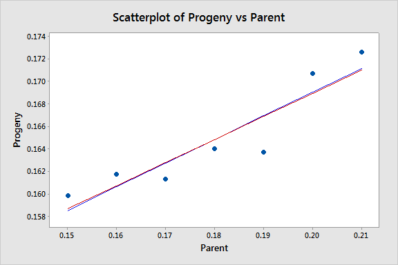
The black line represents the OLS fit, while the red line represents the WLS fit. The standard deviations tend to increase as the value of Parent increases, so the weights tend to decrease as the value of Parent increases. Thus, on the left of the graph where the observations are up-weighted the red fitted line is pulled slightly closer to the data points, whereas on the right of the graph where the observations are down-weighted the red fitted line is slightly further from the data points.
For this example, the weights were known. There are other circumstances where the weights are known:
- If the i-th response is an average of \(n_i\) equally variable observations, then \(Var\left(y_i \right)\) = \(\sigma^2/n_i\) and \(w_i\) = \(n_i\).
- If the i-th response is a total of \(n_i\) observations, then \(Var\left(y_i \right)\) = \(n_i\sigma^2\) and \(w_i\) =1/ \(n_i\).
- If variance is proportional to some predictor \(x_i\), then \(Var\left(y_i \right)\) = \(x_i\sigma^2\) and \(w_i\) =1/ \(x_i\).
In practice, for other types of datasets, the structure of W is usually unknown, so we have to perform an ordinary least squares (OLS) regression first. Provided the regression function is appropriate, the i-th squared residual from the OLS fit is an estimate of \(\sigma_i^2\) and the i-th absolute residual is an estimate of \(\sigma_i\) (which tends to be a more useful estimator in the presence of outliers). The residuals are much too variable to be used directly in estimating the weights, \(w_i,\) so instead we use either the squared residuals to estimate a variance function or the absolute residuals to estimate a standard deviation function. We then use this variance or standard deviation function to estimate the weights.
Some possible variance and standard deviation function estimates include:
- If a residual plot against a predictor exhibits a megaphone shape, then regress the absolute values of the residuals against that predictor. The resulting fitted values of this regression are estimates of \(\sigma_{i}\). (And remember \(w_i = 1/\sigma^{2}_{i}\)).
- If a residual plot against the fitted values exhibits a megaphone shape, then regress the absolute values of the residuals against the fitted values. The resulting fitted values of this regression are estimates of \(\sigma_{i}\).
- If a residual plot of the squared residuals against a predictor exhibits an upward trend, then regress the squared residuals against that predictor. The resulting fitted values of this regression are estimates of \(\sigma_{i}^2\).
- If a residual plot of the squared residuals against the fitted values exhibits an upward trend, then regress the squared residuals against the fitted values. The resulting fitted values of this regression are estimates of \(\sigma_{i}^2\).
After using one of these methods to estimate the weights, \(w_i\), we then use these weights in estimating a weighted least squares regression model. We consider some examples of this approach in the next section.
Some key points regarding weighted least squares are:
- The difficulty, in practice, is determining estimates of the error variances (or standard deviations).
- Weighted least squares estimates of the coefficients will usually be nearly the same as the "ordinary" unweighted estimates. In cases where they differ substantially, the procedure can be iterated until estimated coefficients stabilize (often in no more than one or two iterations); this is called iteratively reweighted least squares.
- In some cases, the values of the weights may be based on theory or prior research.
- In designed experiments with large numbers of replicates, weights can be estimated directly from sample variances of the response variable at each combination of predictor variables.
- The use of weights will (legitimately) impact the widths of statistical intervals.