Previously in Lesson 4, we mentioned two measures that we use to help identify outliers. They are:
- Residuals
- Studentized residuals (or internally studentized residuals) (which Minitab calls standardized residuals)
We briefly review these measures here. However, this time, we add a little more detail.
Residuals
As you know, ordinary residuals are defined for each observation, i = 1, ..., n as the difference between the observed and predicted responses:
\(e_i=y_i-\hat{y}_i\)
For example, consider the following very small (contrived) data set containing n = 4 data points (x, y).
| x | y | FITS | RESI |
|---|---|---|---|
| 1 | 2 | 2.2 | -0.2 |
| 2 | 5 | 4.4 | 0.6 |
| 3 | 6 | 6.6 | -0.6 |
| 4 | 9 | 8.8 | 0.2 |
The column labeled "FITS" contains the predicted responses, while the column labeled "RESI" contains the ordinary residuals. As you can see, the first residual (-0.2) is obtained by subtracting 2.2 from 2; the second residual (0.6) is obtained by subtracting 4.4 from 5; and so on.
As you know, the major problem with ordinary residuals is that their magnitude depends on the units of measurement, thereby making it difficult to use the residuals as a way of detecting unusual y values. We can eliminate the units of measurement by dividing the residuals by an estimate of their standard deviation, thereby obtaining what is known as studentized residuals (or internally studentized residuals) (which Minitab calls standardized residuals).
Studentized residuals (or internally studentized residuals)
Studentized residuals (or internally studentized residuals) are defined for each observation, i = 1, ..., n as an ordinary residual divided by an estimate of its standard deviation:
\(r_{i}=\dfrac{e_{i}}{s(e_{i})}=\dfrac{e_{i}}{\sqrt{MSE(1-h_{ii})}}\)
Here, we see that the internally studentized residual for a given data point depends not only on the ordinary residual but also on the size of the mean square error (MSE) and the leverage \(h_{ii}\).
For example, consider again the (contrived) data set containing n = 4 data points (x, y):
| x | y | FITS | RESI | HI | SRES |
|---|---|---|---|---|---|
| 1 | 2 | 2.2 | -0.2 | 0.7 | -0.57735 |
| 2 | 5 | 4.4 | 0.6 | 0.3 | 1.13389 |
| 3 | 6 | 6.6 | -0.6 | 0.3 | -1.13389 |
| 4 | 9 | 8.8 | 0.2 | 0.7 | 0.57735 |
The column labeled "FITS" contains the predicted responses, the column labeled "RESI" contains the ordinary residuals, the column labeled "HI" contains the leverages \(h_{ii}\), and the column labeled "SRES" contains the internally studentized residuals (which Minitab calls standardized residuals). The value of MSE is 0.40. Therefore, the first internally studentized residual (-0.57735) is obtained by:
\(r_{1}=\dfrac{-0.2}{\sqrt{0.4(1-0.7)}}=-0.57735\)
and the second internally studentized residual is obtained by:
\(r_{2}=\dfrac{0.6}{\sqrt{0.4(1-0.3)}}=1.13389\)
and so on.
The good thing about internally studentized residuals is that they quantify how large the residuals are in standard deviation units, and therefore can be easily used to identify outliers:
- An observation with an internally studentized residual that is larger than 3 (in absolute value) is generally deemed an outlier. (Sometimes, the term "outlier" is reserved for observation with an externally studentized residual that is larger than 3 in absolute value—we consider externally studentized residuals in the next section.)
- Recall that Minitab flags any observation with an internally studentized residual that is larger than 2 (in absolute value).
Minitab may be a little conservative, but perhaps it is better to be safe than sorry. The key here is not to take the cutoffs of either 2 or 3 too literally. Instead, treat them simply as red warning flags to investigate the data points further.
Example 11-2 Revisited Section
Let's take another look at the following Influence2 data set
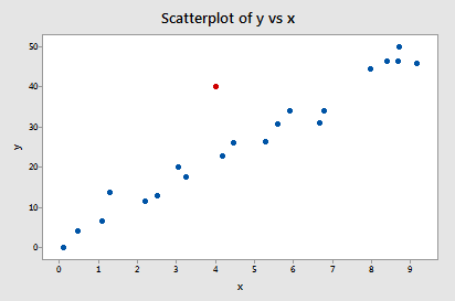
In our previous look at this data set, we considered the red data point an outlier, because it does not follow the general trend of the rest of the data. Let's see what the internally studentized residual of the red data point suggests:
Fits and Diagnostics for Unusual Observations
| Obs | y | Fit | Resid | Std Resid | |
|---|---|---|---|---|---|
| 21 | 40.00 | 23.11 | 16.89 | 3.68 | R |
R Large residual
Indeed, its internally studentized residual (3.68) leads Minitab to flag the data point as being an observation with a "Large residual." Note that Minitab labels internally studentized residuals as "Std Resid" because it refers to such residuals as "standardized residuals."
Why should we care about outliers? Section
We sure spend an awful lot of time worrying about outliers. But, why should we? What impact does their existence have on our regression analyses? One easy way to learn the answer to this question is to analyze a data set twice—once with and once without the outlier—and to observe differences in the results.
Let's try doing that to our Example #2 data set. If we regress y on x using the data set without the outlier, we obtain:
Analysis of Variance
| Source | DF | Seq SS | Seq MS | F-Value | P-Value |
|---|---|---|---|---|---|
| Regression | 1 | 4386.1 | 4386.07 | 652.84 | 0.000 |
| x | 1 | 4386.1 | 4386.07 | 652.84 | 0.000 |
| Error | 18 | 120.9 | 6.72 | ||
| Total | 19 | 4507.0 |
Modal Summary
| S | R-sq | R-sq(adj) | R-sq(pred) |
|---|---|---|---|
| 2.59199 | 97.32% | 91.17% | 96.63% |
Regression Equation
\(\widehat{y}= 1.3 + 5.117x\)
And if we regress y on x using the full data set with the outlier, we obtain:
Analysis of Variance
| Source | DF | Seq SS | Seq MS | F-Value | P-Value |
|---|---|---|---|---|---|
| Regression | 1 | 4265.8 | 4265.82 | 192.23 | 0.000 |
| x | 1 | 4265.8 | 4265.82 | 192.23 | 0.000 |
| Error | 19 | 421.6 | 22.19 | ||
| Total | 20 | 4687.5 |
Modal Summary
| S | R-sq | R-sq(adj) | R-sq(pred) |
|---|---|---|---|
| 4.71075 | 91.01% | 90.53% | 89.61% |
Regression Equation
\(\widehat{y}= 2.96 + 5.037x\)
What aspect of the regression analysis changes substantially because of the existence of the outlier? Did you notice that the mean square error MSE is substantially inflated from 6.72 to 22.19 by the presence of the outlier? Recalling that MSE appears in all of our confidence and prediction interval formulas, the inflated size of MSE would thereby cause a detrimental increase in the width of all of our confidence and prediction intervals. However, as noted in Section 11.1, the predicted responses, estimated slope coefficients, and hypothesis test results are not affected by the inclusion of the outlier. Therefore, the outlier, in this case, is not deemed influential (except with respect to MSE).