Okay, now that we know the effects that multicollinearity can have on our regression analyses and subsequent conclusions, how do we tell when it exists? That is, how can we tell if multicollinearity is present in our data?
Some of the common methods used for detecting multicollinearity include:
- The analysis exhibits the signs of multicollinearity — such as estimates of the coefficients varying from model to model.
- The t-tests for each of the individual slopes are non-significant (P > 0.05), but the overall F-test for testing all of the slopes is simultaneously 0 is significant (P < 0.05).
- The correlations among pairs of predictor variables are large.
Looking at correlations only among pairs of predictors, however, is limiting. It is possible that the pairwise correlations are small, and yet a linear dependence exists among three or even more variables, for example, \(X_3 = 2X_1 + 5X_2 + \text{error}\), say. That's why many regression analysts often rely on what is called variance inflation factors (VIF) to help detect multicollinearity.
What is a Variation Inflation Factor? Section
As the name suggests, a variance inflation factor (VIF) quantifies how much the variance is inflated. But what variance? Recall that we learned previously that the standard errors — and hence the variances — of the estimated coefficients are inflated when multicollinearity exists. So, the variance inflation factor for the estimated coefficient \(b_k\) — denoted \(VIF_k\) — is just the factor by which the variance is inflated.
Let's be a little more concrete. For the model in which \(x_k\) is the only predictor:
\(y_i=\beta_0+\beta_kx_{ik}+\epsilon_i\)
it can be shown that the variance of the estimated coefficient \(b_k\) is:
\(Var(b_k)_{min}=\dfrac{\sigma^2}{\sum_{i=1}^{n}(x_{ik}-\bar{x}_k)^2}\)
Note that we add the subscript "min" in order to denote that it is the smallest the variance can be. Don't worry about how this variance is derived — we just need to keep track of this baseline variance, so we can see how much the variance of \(b_k\) is inflated when we add correlated predictors to our regression model.
Let's consider such a model with correlated predictors:
\(y_i=\beta_0+\beta_1x_{i1}+ \cdots + \beta_kx_{ik}+\cdots +\beta_{p-1}x_{i, p-1} +\epsilon_i\)
Now, again, if some of the predictors are correlated with the predictor \(x_k\), then the variance of \(b_k\) is inflated. It can be shown that the variance of \(b_k\) is:
\(Var(b_k)=\dfrac{\sigma^2}{\sum_{i=1}^{n}(x_{ik}-\bar{x}_k)^2}\times \dfrac{1}{1-R_{k}^{2}}\)
where \(R_{k}^{2}\) is the \(R^{2} \text{-value}\) obtained by regressing the \(k^{th}\) predictor on the remaining predictors. Of course, the greater the linear dependence among the predictor \(x_k\) and the other predictors, the larger the \(R_{k}^{2}\) value. And, as the above formula suggests, the larger the \(R_{k}^{2}\) value, the larger the variance of \(b_k\).
How much larger? To answer this question, all we need to do is take the ratio of the two variances. By doing so, we obtain:
\(\dfrac{Var(b_k)}{Var(b_k)_{min}}=\dfrac{\left( \frac{\sigma^2}{\sum(x_{ik}-\bar{x}_k)^2}\times \dfrac{1}{1-R_{k}^{2}} \right)}{\left( \frac{\sigma^2}{\sum(x_{ik}-\bar{x}_k)^2} \right)}=\dfrac{1}{1-R_{k}^{2}}\)
The above quantity is deemed the variance inflation factor for the \(k^{th}\) predictor. That is:
\(VIF_k=\dfrac{1}{1-R_{k}^{2}}\)
where \(R_{k}^{2}\) is the \(R^{2} \text{-value}\) obtained by regressing the \(k^{th}\) predictor on the remaining predictors. Note that a variance inflation factor exists for each of the (p-1) predictors in a multiple regression model.
How do we interpret the variance inflation factors for a regression model? Again, it measures how much the variance of the estimated regression coefficient \(b_k\) is "inflated" by the existence of correlation among the predictor variables in the model. A VIF of 1 means that there is no correlation between the \(k^{th}\) predictor and the remaining predictor variables, and hence the variance of \(b_k\) is not inflated at all. The general rule of thumb is that VIFs exceeding 4 further warrant investigation, while VIFs exceeding 10 are signs of serious multicollinearity requiring correction.
Example 12-2 Section
Let's return to the Blood Pressure data set in which researchers observed the following data on 20 individuals with high blood pressure:
- blood pressure (y = BP, in mm Hg)
- age (\(x_{1} \) = Age, in years)
- weight (\(x_2\) = Weight, in kg)
- body surface area (\(x_{3} \) = BSA, in sq m)
- duration of hypertension (\(x_{4} \) = Dur, in years)
- basal pulse (\(x_{5} \) = Pulse, in beats per minute)
- stress index (\(x_{6} \) = Stress)
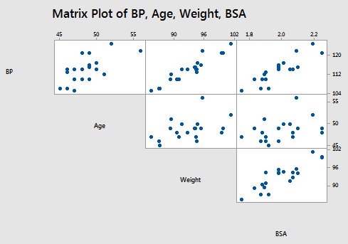
As you may recall, the matrix plot of BP, Age, Weight, and BSA:
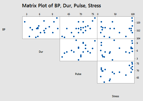
the matrix plot of BP, Dur, Pulse, and Stress:
and the correlation matrix:
Correlation: BP, Age, Weight, BSA, Dur, Pulse, Stress
| BP | Age | Weight | BSA | Due | Pulse | |
|---|---|---|---|---|---|---|
| Age | 0.659 | |||||
| Weight | 0.950 | 0.407 | ||||
| BSA | 0.866 | 0.378 | 0.875 | |||
| Dur | 0.293 | 0.344 | 0.201 | 0.131 | ||
| Pulse | 0.721 | 0.619 | 0.659 | 0.465 | 0.402 | |
| Stress | 0.164 | 0.368 | 0.034 | 0.018 | 0.312 | 0.506 |
suggest that some of the predictors are at least moderately marginally correlated. For example, body surface area (BSA) and weight are strongly correlated (r = 0.875), and weight and pulse are fairly strongly correlated (r = 0.659). On the other hand, none of the pairwise correlations among age, weight, duration, and stress are particularly strong (r < 0.40 in each case).
Regressing y = BP on all six of the predictors, we obtain:
Analysis of Variance
| Source | DF | Seq SS | Seq MS | F-Value | P-Value |
|---|---|---|---|---|---|
| Regression | 6 | 557.844 | 92.974 | 56.64 | 0.000 |
| Age | 1 | 243.266 | 243.266 | 1466.91 | 0.000 |
| Weight | 1 | 311.910 | 311.910 | 1880.84 | 0.000 |
| BSA | 1 | 1.768 | 1.768 | 10.66 | 0.006 |
| Dur | 1 | 0.335 | 0.335 | 2.02 | 0.179 |
| Pulse | 1 | 0.123 | 0.123 | 0.74 | 0.405 |
| Stress | 1 | 0.442 | 0.442 | 2.67 | 0.126 |
| Error | 13 | 2.156 | 0.166 | ||
| Total | 19 | 560.00 |
Modal Summary
| S | R-sq | R-sq(adj) | R-sq(pred) |
|---|---|---|---|
| 0.407229 | 99.62% | 99.44% | 99.08% |
Coefficients
| Term | Coef | SE Coef | T-Value | P-Value | VIF |
|---|---|---|---|---|---|
| Constant | -12.87 | 2.56 | -5.03 | 0.000 | |
| Age | 0.7033 | 0.0496 | 14.18 | 0.000 | 1.76 |
| Weight | 0.9699 | 0.0631 | 15.37 | 0.000 | 8.42 |
| BSA | 3.78 | 1.58 | 2.39 | 0.033 | 5.33 |
| Dur | 0.0684 | 0.0484 | 1.41 | 0.182 | 1.24 |
| Pulse | -0.0845 | 0.0516 | -1.64 | 0.126 | 4.41 |
| Stress | 0.00557 | 0.00341 | 1.63 | 0.126 | 1.83 |
Minitab reports the variance inflation factors by default. As you can see, three of the variance inflation factors — 8.42, 5.33, and 4.41 — are fairly large. The VIF for the predictor Weight, for example, tells us that the variance of the estimated coefficient of Weight is inflated by a factor of 8.42 because Weight is highly correlated with at least one of the other predictors in the model.
For the sake of understanding, let's verify the calculation of the VIF for the predictor Weight. Regressing the predictor \(x_2\) = Weight on the remaining five predictors:
Analysis of Variance
| Source | DF | Seq SS | Seq MS | F-Value | P-Value |
|---|---|---|---|---|---|
| Regression | 5 | 308.839 | 61.768 | 20.77 | 0.000 |
| Age | 1 | 15.04 | 15.04 | 0.50 | 0.490 |
| BSA | 1 | 212.734 | 212.734 | 71.53 | 0.000 |
| Dur | 1 | 1.442 | 1.442 | 0.48 | 0.498 |
| Pulse | 1 | 27.311 | 27.311 | 9.18 | 0.009 |
| Stress | 1 | 41.639 | 2.974 | ||
| Error | 14 | 41.639 | 2.974 | ||
| Total | 19 | 350.478 |
Modal Summary
| S | R-sq | R-sq(adj) | R-sq(pred) |
|---|---|---|---|
| 1.72459 | 88.12% | 83.88% | 74.77% |
Coefficients
| Term | Coef | SE Coef | T-Value | P-Value | VIF |
|---|---|---|---|---|---|
| Constant | 19.67 | 9.46 | 2.08 | 0.057 | |
| Age | -0.145 | 0.206 | -0.70 | 0.495 | 1.70 |
| BSA | 21.42 | 3.46 | 6.18 | 0.000 | 1.43 |
| Dur | 0.009 | 0.205 | 0.04 | 0.967 | 1.24 |
| Pulse | 0.558 | 0.160 | 3.49 | 0.004 | 2.36 |
| Stress | -0.0230 | 0.0131 | -1.76 | 0.101 | 1.50 |
Minitab reports that \(R_{Weight}^{2}\) is 88.1% or, in decimal form, 0.881. Therefore, the variance inflation factor for the estimated coefficient Weight is by definition:
\(VIF_{Weight}=\dfrac{Var(b_{Weight})}{Var(b_{Weight})_{min}}=\dfrac{1}{1-R_{Weight}^{2}}=\dfrac{1}{1-0.881}=8.4\)
Again, this variance inflation factor tells us that the variance of the weight coefficient is inflated by a factor of 8.4 because Weight is highly correlated with at least one of the other predictors in the model.
So, what to do? One solution to dealing with multicollinearity is to remove some of the violating predictors from the model. If we review the pairwise correlations again:
Correlation: BP, Age, Weight, BSA, Dur, Pulse, Stress
| BP | Age | Weight | BSA | Dur | Pulse | |
|---|---|---|---|---|---|---|
| Age | 0.659 | |||||
| Weight | 0.950 | 0.407 | ||||
| BSA | 0.866 | 0.378 | 0.875 | |||
| Dur | 0.293 | 0.344 | 0.201 | 0.131 | ||
| Pulse | 0.721 | 0.619 | 0.659 | 0.465 | 0.402 | |
| Stress | 0.164 | 0.368 | 0.034 | 0.018 | 0.312 | 0.506 |
we see that the predictors Weight and BSA are highly correlated (r = 0.875). We can choose to remove either predictor from the model. The decision of which one to remove is often a scientific or practical one. For example, if the researchers here are interested in using their final model to predict the blood pressure of future individuals, their choice should be clear. Which of the two measurements — body surface area or weight — do you think would be easier to obtain?! If weight is an easier measurement to obtain than body surface area, then the researchers would be well-advised to remove BSA from the model and leave Weight in the model.
Reviewing again the above pairwise correlations, we see that the predictor Pulse also appears to exhibit fairly strong marginal correlations with several of the predictors, including Age (r = 0.619), Weight (r = 0.659), and Stress (r = 0.506). Therefore, the researchers could also consider removing the predictor Pulse from the model.
Let's see how the researchers would do. Regressing the response y = BP on the four remaining predictors age, weight, duration, and stress, we obtain:
Analysis of Variance
| Source | DF | Seq SS | Seq MS | F-Value | P-Value |
|---|---|---|---|---|---|
| Regression | 4 | 555.455 | 138.864 | 458.28 | 0.000 |
| Age | 1 | 243.266 | 243.266 | 802.84 | 0.000 |
| Weight | 1 | 311.910 | 311.910 | 1029.38 | 0.000 |
| Dur | 1 | 0.178 | 0.178 | 0.59 | 0.455 |
| Stress | 1 | 0.100 | 0.100 | 0.33 | 0.573 |
| Error | 15 | 4.545 | 0.303 | ||
| Total | 19 | 560.000 |
Modal Summary
| S | R-sq | R-sq(adj) | R-sq(pred) |
|---|---|---|---|
| 0.550462 | 99.19% | 98.97% | 98.59% |
Coefficients
| Term | Coef | SE Coef | T-Value | P-Value | VIF |
|---|---|---|---|---|---|
| Constant | -15.87 | 3.20 | -4.97 | 0.000 | |
| Age | 0.6837 | 0.0612 | 11.17 | 0.000 | 1.47 |
| Weight | 1.0341 | 0.0327 | 31.65 | 0.000 | 1.23 |
| Dur | 0.0399 | 0.0645 | 0.62 | 0.545 | 1.20 |
| Stress | 0.00218 | 0.00379 | 0.58 | 0.573 | 1.24 |
Aha — the remaining variance inflation factors are quite satisfactory! That is, it appears as if hardly any variance in inflation remains. Incidentally, in terms of the adjusted \(R^{2} \text{-value}\), we did not seem to lose much by dropping the two predictors BSA and Pulse from our model. The adjusted \(R^{2} \text{-value}\) decreased to only 98.97% from the original adjusted \(R^{2} \text{-value}\) of 99.44%.
Try it!
Variance inflation factors Section
Detecting multicollinearity using \(VIF_k\).
We’ll use the Cement data set to explore variance inflation factors. The response y measures the heat evolved in calories during the hardening of cement on a per gram basis. The four predictors are the percentages of four ingredients: tricalcium aluminate (\(x_{1} \)), tricalcium silicate (\(x_2\)), tetracalcium alumino ferrite (\(x_{3} \)), and dicalcium silicate (\(x_{4} \)). It’s not hard to imagine that such predictors would be correlated in some way.
-
Use the Stat >> Basic Statistics >> Correlation ... command in Minitab to get an idea of the extent to which the predictor variables are (pairwise) correlated. Also, use the Graph >> Matrix Plot ... command in Minitab to get a visual portrayal of the (pairwise) relationships among the response and predictor variables.
There’s a strong negative correlation between \(X_2\) and \(X_4\) (-0.973) and between \(X_1\) and \(X_3\) (-0.824). The remaining pairwise correlations are all quite low.
-
Regress the fourth predictor, \(x_4\), on the remaining three predictors, \(x_{1} \), \(x_2\), and \(x_{3} \). That is, fit the linear regression model treating \(x_4\) as the response and \(x_{1} \), \(x_2\), and \(x_{3} \) as the predictors. What is the \({R^2}_4\) value? (Note that Minitab rounds the \(R^{2} \) value it reports to three decimal places. For the purposes of the next question, you’ll want a more accurate \(R^{2} \) value. Calculate the \(R^{2} \) value SSR using its definition, \(\dfrac{SSR}{SSTO}\). Use your calculated value, carried out to 5 decimal places, in answering the next question.)
\(R^2 = SSR/SSTO = 3350.10/3362.00 = 0.99646\)
-
Using your calculated \(R^{2} \) value carried out to 5 decimal places, determine by what factor the variance of \(b_4\) is inflated. That is, what is \(VIF_4\)?
\(VIF_4 = 1/(1-0.99646) - 282.5\) -
Minitab will actually calculate the variance inflation factors for you. Fit the multiple linear regression model with y as the response and \(x_{1} \),\(x_2\),\(x_{3} \) and \(x_{4} \) as the predictors. The \(VIF_k\) will be reported as a column of the estimated coefficients table. Is the \(VIF_4\) that you calculated consistent with what Minitab reports?
\(VIF_4 = 282.51\)
-
Note that all of the \(VIF_k\) are larger than 10, suggesting that a high degree of multicollinearity is present. (It should seem logical that multicollinearity is present here, given that the predictors are measuring the percentage of ingredients in the cement.) Do you notice anything odd about the results of the t-tests for testing the individual \(H_0 \colon \beta_i = 0\) and the result of the overall F-test for testing \(H_0 \colon \beta_1 = \beta_2 = \beta_3 = \beta_4 = 0\)? Why does this happen?
The individual t-tests indicate that none of the predictors are significant given the presence of all the others, but the overall F-test indicates that at least one of the predictors is useful. This is a result of the high degree of multicollinearity between all the predictors.
-
We learned that one way of reducing data-based multicollinearity is to remove some of the violating predictors from the model. Fit the linear regression model with y as the response and \(X_1\) and \(X_2\) as the only predictors. Are the variance inflation factors for this model acceptable?
The VIFs for the model with just \(X_1\) and \(X_2\) are just 1.06 and so are acceptable.